Stanford CS224n Notes

For a few years now, Stanford has offered CS224n, a lecture series on Natural Language Processing with Deep Learning taught by Professor Christopher Manning, one of the top researchers in NLP, on YouTube. I’ve been watching a few of the lectures in my free time, but now, I would like to formally take notes on the lectures to help me gain a deeper understanding of the concepts. I will be posting my notes here, and if you would like to follow along, you can find the lectures here

Lecture 1: Introduction and Word Vectors §

How do we represent the meaning of a word §

• Linguists define denotational semantics as the isomorphic relation between the signifier (which is the word/symbol) and the signified (idea or thing).
• How is this implemented in traditional NLP:
  • WordNet: a thesaurus that contains sets of words with their corresponding synonyms, antonyms and hyponyms.
  • The problems with using WordNet to get meaning of words:
    • Not scalable because it was human constructed
    • Missing nuances in the meaning of words
    • Cannot compute good word similarity
  • Traditional NLP uses words as discrete symbols:
    • This means words get one-hot encoding vectors, where each word has its own dimension
    • $v_{natural}=\left(\begin{array}{ccccccc}0& 0& \dots & 1& \dots & 0& 0\end{array}\right)$
    • an example can be seen above, where the word natural is represented by a vector where every dimension has a zero in it except for one, which happens to be the dimension for natural.
    • Problems with this:
      • Dimensionality becomes to large, and there is no natural notion of similarity between words
• Instead of using denotational semantics, we can attempt to use distributional semantics
  • This means a word’s meaning is given by the words that appear around it frequently
  • This is used to create word vectors/embeddings:
    • We build up dense vectors for each word in an embedding space such that in this space, words that have similar meaning appear close to each other in this space.
• This is the motivation behind word2vec

“You shall know a word by the company it keeps” - J.R. Firth

word2vec Overview §

• You are give a large corpus of text (i.e. all wikipedia pages)
• You will have every word in a fixed vocabulary $w$ represented by a vector $v_w$.
• Go through each position $t$ in the text, with center word $c$ and context words $o$, where the context words are the words that appear to the left and right of the center word at a fixed window size.
• You are to calculate $p(o|c)$ (or vise versa), and you’re goal is to adjust the word vectors to maximize these probabilities. It is a Maximum Likelihood objective.
• Example:
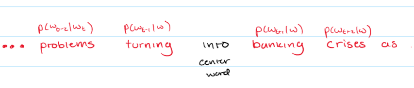
• In this example, you see that the center word is into, and the surrounding words are the context words, and you are calculating $p(w_{t-2}|w_t),p(w_{t-1}|w_t),\dots$ .

Objective Function §

• For each position $t=1,2,\dots ,T$, predict the context words within a window of fixed size $m$ given a center word $w_t$.
  • $L(\theta )={\prod }_{t=1}^T{\prod }_{-m<j<m}P(w_{t+j}|w_t;\theta )$ where $\theta$ are all of our word vectors that we are trying to optimize.
  • To make the math simpler, we take the negative log of this function to get our final objective function
  • $J(\theta )=-\frac{1}{T}{\sum }_{t=1}^T{\sum }_{-m<j<m}\log (P(w_{t+j}|w_t;\theta ))$
  • We want to minimize this objective function
• How do we calculate $P(w_{t+j}|w_t;\theta )$?
  • We allocate two vectors per word $w$:
    • $v_w$ is when $w$ is the center word
    • $u_w$ is when a(n) outside/context word.
  • Probability of a context word $o$ given a center word $c$ :
    • $P(o|c)=\frac{exp(u_o^T\ast v_c)}{{\sum }_{w\in V}exp(u_w^T\ast v_c)}$
    • You take the dot product of the context word and the center word (larger dot product $\to$ larger probability)
    • The denominator is used to normalize over the entire vocabulary to create a probability distribution.

Training the Model §

• We want to optimize the parameters to minimize loss
• $\theta$ represents all the model’s parameters (i.e all the word vectors):
  • $\theta =\left[\begin{array}{c}{v}_{aardvark}\\ v_a\\ ⋮\\ v_{zebra}\\ u_{aardvark}\\ ⋮\\ u_{zebra}\end{array}\right]\in {\mathbb{R}}^{2dV}$
  • We have 2 d-dimensional vectors for all V words in dictionary.
• We can then use gradient descent :
  • The loss function is, again $J(\theta )=-\frac{1}{T}{\sum }_{t=1}^T{\sum }_{-m<j<m}\log (P(w_{t+j}|w_t;\theta ))$. After plugging in the necessary equations, we find that:
  • $\frac{\partial }{\partial v_c}J(\theta )=u_o-{\sum }_{x=1}^{V}p(x|c)\ast u_x$
  • This equation tells us that the derivative is basically the observed - expected for context words.
• General equations for Gradient Descent:
  • ${\theta }^{new}={\theta }^{old}-\alpha {\nabla }_{\delta }J(\theta )$ (this is matrix notation, and $\alpha$ is the learning rate, which is a hyperparameter)
  • For element-wise:
  • ${\theta }_j^{new}={\theta }_j^{old}-\alpha \frac{\partial }{\partial {\theta }_j}J(\theta )$
• Stochastic Gradient Descent:
  • Computing the gradient over the full corpus is an expensive task
  • Instead we can use Stochastic gradient descent by estimating the gradient based on small batches of the corpus.
  • With the word vectors, the gradients should be very sparse at each iteration because you don’t see most words in each batch. This means you will only update the words that actually appear in the batch.

Capturing Co-Occurrence Matrix §

• Each vector has counts on how many times each word occurs near other words.
• You can build co-occurrence matrices using windows similar to word2vec on a corpus.
• These become sparse and large in dimensionality.
• You can reduce the dimensionality of the Co-Occurrence vectors using singular value decomposition. You retain $k$ singular values to get a rank $k$ approximation of the co-occurrence matrix.

GloVe Algorithm §

• You want to combine the use of count based methods (because they provide fast training and efficient statistics) and direct prediction methods (because easier to scale and generally work better).
• We encode meaning components in vector differences
  • A crucial insight: The ratios of co-occurrence probabilities can encode meaning components of a word.
• You can encode linear meaning components into the word vectors.

How to evaluate word vectors §

• Intrinsic Evaluations:
  • Evaluation on specific/intermediate subtasks
  • These evaluations are fast to compute
  • There is a correlation between performance in these tests and actual real tasks.
• Extrinsic:
  • Evaluation on real tasks
  • Long time to compute.

Summary §

Word vectors are numerical representations of words that, unlike bag-of-words representations, can encode semantic relationships between words in a continuous vector space. Additionally, word vectors are generally smaller in dimension compared to bag-of-words representations, which makes computations more efficient.

Word2vec is a popular word vector algorithm. It uses a neural architecture to learn word representations from a large corpus of text by predicting the likelihood of a context word given a center word.

Lecture 2: Backpropagation and Neural Networks §

* I cover most of this lecture in my Backpropagation Article. *

Parts I Didn’t Cover §

Regularization §

• Regularization is a technique used to prevent overfitting in machine learning models. One way of implementing this is modifying the cost function to the following: $J(\theta )=\frac{1}{N}{\sum }_{i=1}^N-\log (\frac{e^{f_{y_i}}}{\sum e^{f_c}})+\lambda {\sum }_k{\theta }_k^2$ This modification adds a term to the cost function that will penalize large values of the parameters $\theta$.

Dropout §

• Dropout is a more common regularization technique that is used in neural networks.
• At each training step, we randomly set 50% of the inputs to each neuron to 0, which will thereby prevent the neuron from being activated.
• This prevents the network from relying on any one neuron, and forces it to learn more robust representations.

Other Notes §

• Initialize all the weights to random values
• Adam optimizer is usually the best.

Lecture 3: Recurrent Neural Networks and Language Models §

What is Language Modeling? §

• Language modeling is the task of predicting what word comes next in a sequence of words.
• Ex: “The students opened their ________”
• More formally:
  • Given a sequence of words $w_1,w_2,\dots ,w_n$, compute the probability distribution of the next word $w_{n+1}$. $P(w_{n+1}|w_1,w_2,\dots ,w_n)$ $x_{n+1}\in V=\{x_1,x_2,\dots ,x_{|V|}\}$
• N-Gram Language Models
  • An N-Gram is a chunk of N consecutive words.
  • Idea: Collect the statistics of how frequent different N-grams occur in a large corpus of text and build a probability distribution over the next word based on the N-gram that precedes it.
  • This is based in the Markovian Assumption, which states that the probability of $x_{n+1}$ only depends on the previous N-1 words.
  • Sparsity Problem:
    • There is a large probability that a specific sequence of words will never occur in a corpus, and as $N$ increases, the probability of this happening increases exponentially.
  • Storage Problem:
    • Storing all the possible N-Grams takes too much storage
• Neural Language Models:
  • We can take the Markovian Assumption of the N-Gram model and apply the same idea to a neural network with word embeddings as seen below:
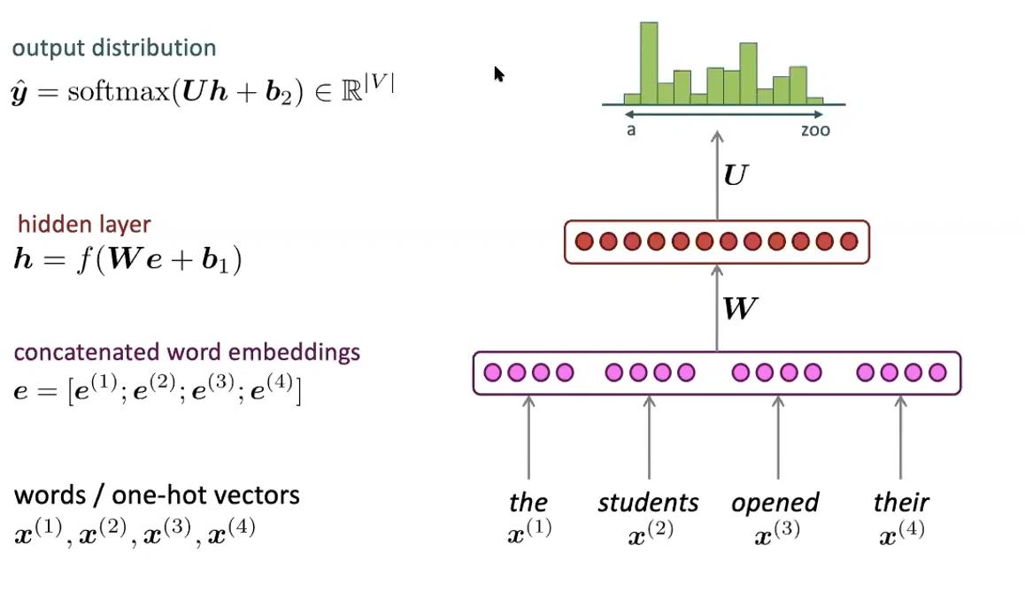
  • The neural network takes a fixed window of N words as inputs and feeds their word embeddings into a neural network. The output of the neural network is a probability distribution over the entire vocabulary.
  • This allows distributed representations of words, so it solves storage and sparsity problems. It does not allow us to use bigger/variable length context windows, and it does not give us a sense of the order of the words in the sentence.

Recurrent Neural Networks §

• RNNs are a type of neural network that allows us to use variable length context windows and also gives us a sense of the order of the words in the sentence.
• The Basic Idea:
  • We feed in the first word of the sentence in to the network and receive an output vector. We then feed the second word of the sentence into the same network, but we also feed in the output of the hidden layer from the first word. We then receive a new output vector. We continue this process until we have processed the entire sentence. Feeding the output of the hidden layer from the previous word allows us to use the context of the previous words in the sentence.
• Simple RNN:
  • Let $x^{(t)}$ be the input vector at time step $t$, $h^{(t)}$ be the hidden state at time step $t$, and $y^{(t)}$ be the output at time step $t$.
  • ${\hat{y}}^{(t)}=softmax(U{h}^{(t)}+b_2)$
  • $h^{(t)}=\sigma (W_h{h}^{(t-1)}+W_e{e}^{(t)}+b_1)$
  • $e^{(t)}=E{x}^{(t)}$
  • $W_h,W_e,U,b_1,b_2$ are the parameters of the network.
  • $\sigma$ is the sigmoid function.
  • $x^{(t)}$ is the input vector at time step $t$.
• Training an RNN Model:
  • We get a big corpus of text $D=\{x^{(1)},x^{(2)},\dots ,x^{(T)}\}$, and we feed it into an RNN-based language model.
  • At each time step $t$, we compute the distribution over the next word $y^{(t)}$.
  • The loss function will be a cross-entropy loss function between the predicted distribution and the actual distribution: $J(\theta )=-{\sum }_{w\in V}{y}_w^{(t)}\log ({\hat{y}}_w^{(t)})=-\log ({\hat{y}}_w^{(t)})$
  • We average this loss for the entire dataset at each time step.
  • Teacher Forcing:
    • If the model gets a word wrong in the sequence, we don’t want to feed the wrong word back into the model for training. Instead, we feed the correct word back into the model.
  • Computing the gradient across the entire corpus is too expensive:
    • We cut the corpus into batches of sentences and use Stochastic Gradient Descent to train the model in a more computationally efficient manner.
  • Backpropagation Through Time:
    • What is the derivative of $J^{(t)}(\theta )$ with respect to $W_h$?
      • $\frac{\partial J^{(t)}}{\partial W_h}={\sum }_{i=1}^t\frac{\partial J^{(i)}}{\partial W_h}$
      • The gradient with respect to the repeated weight matrix is the sum of the gradient with respect to each time it appears.
      • Each value in the sum will be different because the hidden state at each time step is different, and there is a different upstream gradient at each time step.
• Generating Text with RNN Model:
  • We can use the RNN model to generate text be repeated sampling of the output as the next input

Problems with Recurrent Neural Networks §

• Vanishing and Exploding Gradient Problem:
  • Let’s say we are calculating the gradient of $J^{(k)}(\theta )$ with respect to $h^{(m)}$, such that $m<<k$. We would get the following: $\frac{\partial J^{(k)}}{\partial h^{(m)}}=\frac{\partial J^{(k)}}{\partial h^{(k)}}\frac{\partial h^{(k)}}{\partial h^{(k-1)}}\frac{\partial h^{(k-2)}}{\partial h^{(k-2)}}\dots \frac{\partial h^{(m+1)}}{\partial h^{(m)}}$
  • If all of these partial derivatives are less than 1, then the gradient will be exponentially small, which will prevent the gradient to propagate back to the earlier layers, making it harder for the earlier layers to learn. This is called the vanishing gradient problem.
  • If all of these partial derivatives are greater than 1, then the gradient will be exponentially large, which will cause the gradient to explode and the weights will become too large. If the gradient becomes too large, we can get a bad update and teach a bad parameter. This is called the exploding gradient problem.
    • Exploding gradient has an easy fix: we can just clip the gradient to a maximum value that we decide.
  • Vanishing gradient is a harder problem to solve.
    • We can use Long Short-Term Memory (LSTM) networks to solve this problem.

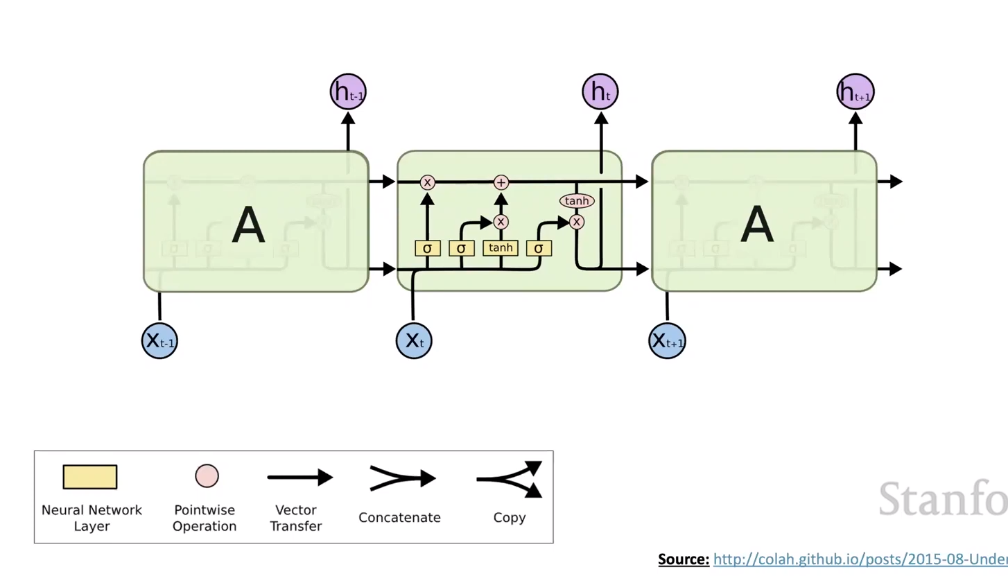
Long Short-Term Memory (LSTM) Networks §

• LSTM Networks are a type of RNN that allow us to “choose” what information to keep and what information to forget as we go from one time step to the next.
• At each time step $t$, there is an input vector $x^{(t)}$, a hidden state $h^{(t)}$, a cell state $c^{(t)}$, and an output vector $y^{(t)}$.
• The cell state:
  • The cell state helps store long-term information, and contains gates such that we can read, erase, and write information to the cell state that we want to.
• At time step $t$, given the input vector $x^{(t)}$:
  • to erase (forget): $f^{(t)}=\sigma (W_f{h}^{(t-1)}+U_f{x}^{(t)}+b_f)$
  • to write: $i^{(t)}=\sigma (W_i{h}^{(t-1)}+U_i{x}^{(t)}+b_i)$
  • to read: $o^{(t)}=\sigma (W_o{h}^{(t-1)}+U_o{x}^{(t)}+b_o)$
• To write new cell content ${\tilde{c}}^{(t)}$:
  • ${\tilde{c}}^{(t)}=tanh(W_c{h}^{(t-1)}+U_c{x}^{(t)}+b_c)$
  • $c^{(t)}=f^{(t)}\odot c^{(t-1)}+i^{(t)}\odot {\tilde{c}}^{(t)}$
  • $h^{(t)}=o^{(t)}\odot tanh(c^{(t)})$ In ${\tilde{c}}^{(t)}$, we are computing the new cell content how we normally would. We multiply the information from the previous hidden state by a weight matrix $W_c$, and we multiply the input vector by a weight matrix $U_c$. We then add a bias $b_c$ and apply the tanh function. After this, to get the new cell state, we perform an element-wise multiplication between the lass cell state with the forget gate $f^{(t)}$ to “forget” information we don’t need. We then add the new cell content ${\tilde{c}}^{(t)}$ multiplied by the write gate $i^{(t)}$ to add the new information. We then compute the new hidden state by multiplying the cell state by the read gate $o^{(t)}$ and applying the tanh function.

Lecture 4: Sequence-to-Sequence Models, Machine Translation and Attention §

Translation §

Statistical Machine Translation §

• Before Neural Machine Translation (NMT), we used Statistical Machine Translation (SMT), which was building probabilistic models from large amounts of data.
• The core objective was ${\mathrm{argmax}}_y\{P(y|x)\}$, where $x$ is the source sentence and $y$ is the target sentence. Using Bayes’ Rule, we get: ${\mathrm{argmax}}_y\{P(y|x)\}={\mathrm{argmax}}_y\{P(x|y)P(y)\}$
• In this case $P(x|y)$ is the translation model, and $P(y)$ is the language model. To learn these models, we would need large amounts of parallel data.
• We would also need to take into account alignment between the source and target sentences because different languages put words in different orders.
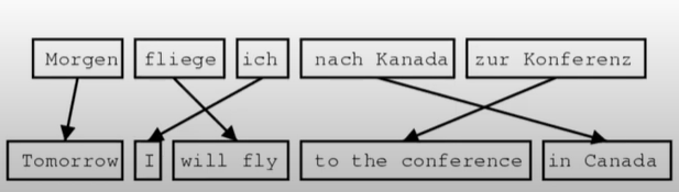
• Taking into account all of this can get really complex.

Neural Machine Translation §

• Neural Machine Translation is the idea of doing machine translation with a single end-to-end neural network.
• This is done using a sequence-to-sequence model.
  • This involves two neural networks: an encoder and a decoder.
  • The encoder takes the source sentence as input and encodes it into a vector, and the decoder takes the vector as input and decodes it into the target sentence.
  • This architecture is very versatile, as it can be used for many tasks:
    • Machine Translation
    • Dialogue
    • Parsing
    • Code Generation
• For Neural Machine Translation with a Recurrent Neural Network Seq2Seq model, the source sentence is passed through the encoder, and the last hidden state of the encoder is the final encoded vector of the source sentence This vector will be passed into the start of the decoder model as context, so it can be used to help generate the target sentence.

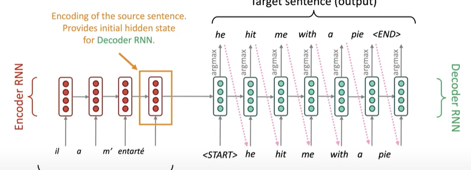
Conditional Language Model §

• The decoder is considered a conditional language model because its objective is to predict the next word in the target sentence given previous words and the context vector from the encoder.

Training Neural Machine Translation Models §

• Training the model will still require large amounts of parallel data.
• The seq2seq model is optimized as one huge system, so all weights are updated at the same time/iteration.
• We take the Cross-Entropy Loss at each time step of the decoder model, and sum them up to get the total loss.
• This loss is then backpropagated through the entire network to update all of the weights, including the encoder.

Decoding Neural Machine Translation Models §

• There are many approaches to performing decoding of the seq2seq model. Decoding is the process of generating the target sentence given the source sentence.
• Greedy Decoding:
  • This is the most intuitive approach to decoding.
  • At each time step, pick the word that has the highest probability of being the next word.
  • This comes with the problem of not being able to undo a decision. Once a decision has been made, it has to be stuck with.
• Exhaustive Search Decoding:
  • We basically try all possible combinations of words and pick the one with the highest probability.
  • This is the complete opposite of greedy decoding. While it may generate a better sentence, it is very computationally expensive, so it is not feasible.
• Beam Search Decoding:
  • This is the middle point between greedy decoding and exhaustive search decoding, and is most commonly used.
  • On each step of the decoder, keep track of the top $k$ most likely sentences and their probabilities.
  • At each time step, only keep the top $k$ most likely sentences, and discard the rest, and keep repeating until all hypotheses reach an ending token.

Advantages and Disadvantages of Neural Machine Translation §

• We generally receive better quality translations than SMT, as there is better use of context and better use of phrase similarities.
• There is also far less engineering effort required
• However, it is not as interpretable, making it harder to debug, and it is difficult to control.

Evaluation of Machine Translation §

• The general standard for measuring performance of machine translation is the BLEU (Bilingual Evaluation Understudy) score.
  • With this, you compare the generated translation with several reference human translations and compute a similarity score.

Difficulties of Machine Translation §

• We have to consider many things:
  • Out-of-vocabulary words
    • There will be words in the source sentence that are not in the vocabulary of the model due to spelling mistakes, slang, etc.
  • Low-Resource Languages
    • There may not be enough data to train a good model for low-resource languages.
  • Gender Biases
    • Gender biases are usually picked up by the model, and it is difficult to remove them.

Attention §

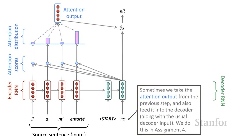
• In regular seq2seq models, there is one core issue: All of the information from the source sentence that the decoder has to use is encoded into a singular vector at the last hidden state. This is an information bottleneck, as the decoder has to use this one vector to generate the entire target sentence.

• Core Idea of Attention: At each step of the decoder, use direct connections to the encoder to focus on particular parts of the source sentence.

Attention in Equations §

• We have hidden states $h_1,h_2,...,h_n\in {\mathbb{R}}^h$ from the encoder.

• At each time step $t$, we have decoder state $s_t\in {\mathbb{R}}^h$.

• Attention scores for each hidden state at this encoder state are computed as follows: $e_t=\left[\begin{array}{c}{s}_t^T{h}_1,s_t^T{h}_2\dots s_t^T{h}_n\end{array}\right]$

• We then apply the softmax function to get the attention weights: ${\alpha }_t=\text{softmax}(e_t)$

• We then compute a weighted sum of the hidden states with the attention weights to get the context vector $a_t$: $a_t={\sum }_{i=1}^n{\alpha }_{t,i}{h}_i$

• We then concatenate the attention vector $a_t$ with the decoder state $s_t$ to get the final context vector $c_t\in {\mathbb{R}}^{2h}$

Advantages of Attention §

• This significantly improves the performance of the model, as it is able to focus on the parts of the source sentence that are most relevant to the current step of the decoder.
• Helps solve information bottleneck problem.
• Helps solve vanishing gradient problem.
• Helps solve long-term dependency problem.
• Provides some form of interpretability.

Lecture 5: Self-Attention and Transformers §

Previously, we looked at Recurrent Neural Networks/Long Short-Term Memory Networks and how they can be used for sequence-to-sequence models paired with attention.

• Encode input sequence into a vector using an encoder such as a Bi-LSTM.
• Feed the encoded vector into a decoder such as an LSTM and attention mechanism to generate the output sequence.
• This creates a seq2seq model that can be used for machine translation, dialogue, parsing, etc.

Problems with this approach:

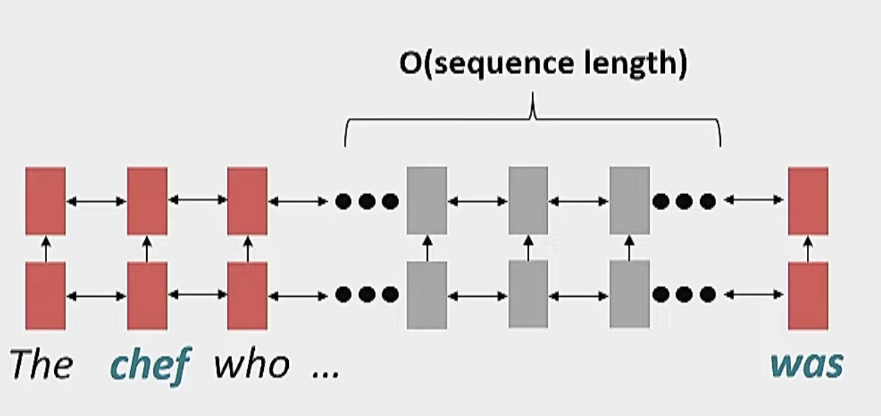
• Linear Interaction Distance:
  • RNN’s encode linear locality, so nearby words affect each others meanings.
  • However, it takes $O(\text{length of sequence})$ for distant pairs of words to interact
  • Makes it hard to learn long-range dependencies
  • Additionally, processing words in order is not always the best way to process them.
• Lack of Parallelism:
  • RNN’s are inherently sequential, so they cannot be parallelized.
  • This makes it hard to train RNN’s on large datasets.
  • This also makes it hard to train RNN’s on GPUs, which are optimized for parallel computation.
• Encoding input all into one vector at the very end creates an information bottleneck.

Possible Solutions:

• Use of Convolutional Neural Networks:

  • Aggregate local contexts using 1D convolutions.
  • This allows for parallelization.
  • Does not solve information bottleneck problem and long range dependency problem.

• Use of Attention:

  • A viable solution that could potentially solve long range dependency problem and information bottleneck problem as well as parallelization problem.

Attention and Self-Attention §

Attention §

• Attention treats each word’s representation as a query to access and incorporate information from a set of values.
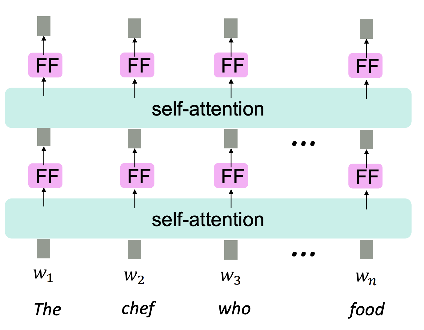
• We can perform attention within a single sequence.
• In the figure, you can see all words attend to all words in previous layer. All of these operations can happen in parallel.
• $O(1)$ interaction distance between any two words.

Attention as a Soft, Averaging Lookup Table §

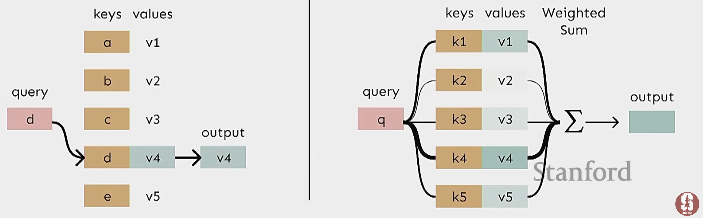
• We can think of attention as a soft, averaging lookup table in a key-value store.
• In a traditional lookup table:
  • The query is input, it finds the matching key, and returns the corresponding value.
• In Attention:
  • Query matches softly to all keys with a weight between 0 and 1, and a weighted sum of the values is returned.

Self-Attention §

• Keys, Queries, and Values all come from the same place.
• Let $W_{1:n}$ be a sequence of words (e.g ‘The cat sat on the mat’).
• Let $x_i$ be the embedding of the $i$ th word in the sequence.
• Transform each word into a query, key, and value using three different weight matrices $Q,K,V$:
  • $q_i=Q{x}_i$
  • $k_i=K{x}_i$
  • $v_i=V{x}_i$
• You can compute the attention weights for each word by taking the dot product of the query and key for each word and applying the softmax function:
  • $e_{ij}=q_i^T{k}_j$
  • ${\alpha }_{ij}=\text{softmax}(e_{ij})$
• The final output for each word is the weighted sum of the values of all words using the affinity scores from attention:
  • $o_i={\sum }_{j=1}^n{\alpha }_{ij}{v}_j$

Problems with Self-Attention and Their Solutions §

• Problem:

  • Self-attention is invariant to the order of the words in the sequence.
  • Example: ‘The cat sat on the mat’ and ‘Mat the on sat cat the’ would have the same attention weights.

• Solution:

  • Add positional encodings to the input embeddings.
  • There will be a $p_i$ positional encoding for each word $x_i$.
  • $\widetilde{x_i}=x_i+p_i$
  • $p_i$ could be a sinusoid function of the position of the word in the sequence. $p_i=\left[\begin{array}{c}\sin (\frac{i}{10000^{0/2d}})\\ \cos (\frac{i}{10000^{0/2d}})\\ ⋮\\ \sin (\frac{i}{10000^{(d-1)/2d}})\\ \cos (\frac{i}{10000^{(d-1)/2d})}\end{array}\right]$
  • Position matrix can also be a learned parameter matrix.

• Problem:

  • With attention, there are no non-linearities in the transformation

• Solution:

  • Put a feed-forward MLP network after each attention layer.

• Problem:

  • For tasks such as machine translation and language modeling, you should not be able to look at the future words in the sequence.

• Solution:

  • We mask out attention weights for future words by setting the attention weights for future words to $-\infty$.

All Necessities for Self-Attention §

• Self-Attention: the basis of the method
• Positional Encoding
• Non-Linearities
• Masking

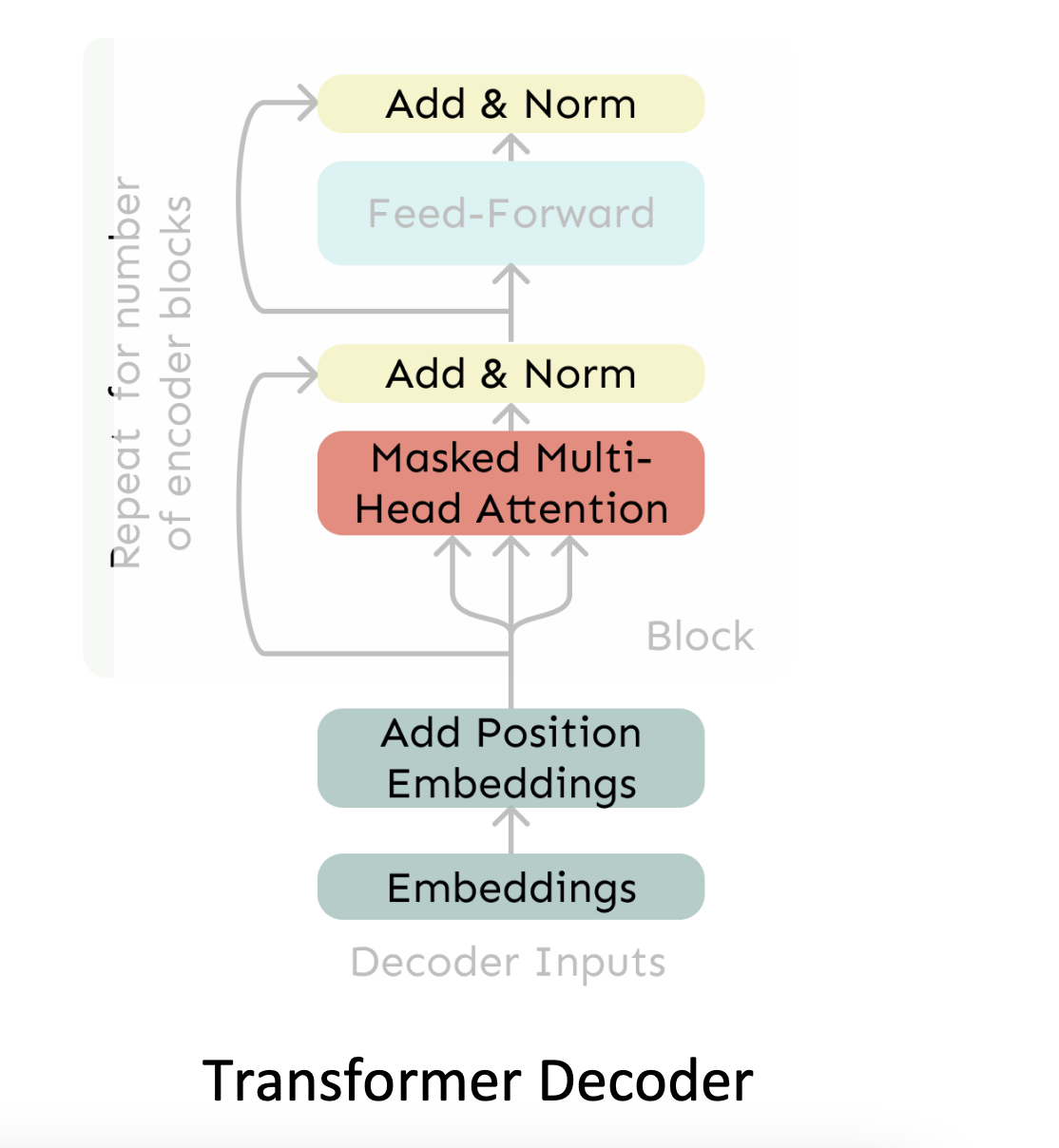
Transformers §

• Transformer decoder used to build language models.
• Very similar to self-attention block, but with a few differences:

Multi-Head Self-Attention §

• There are multiple attention heads with their own Key, Query, Value matrices, so there are different ways to look at different words in a sequence. (e.g. one head can look at the subject, one can look at the object, etc.)

Implementing Multi-Head Self-Attention §

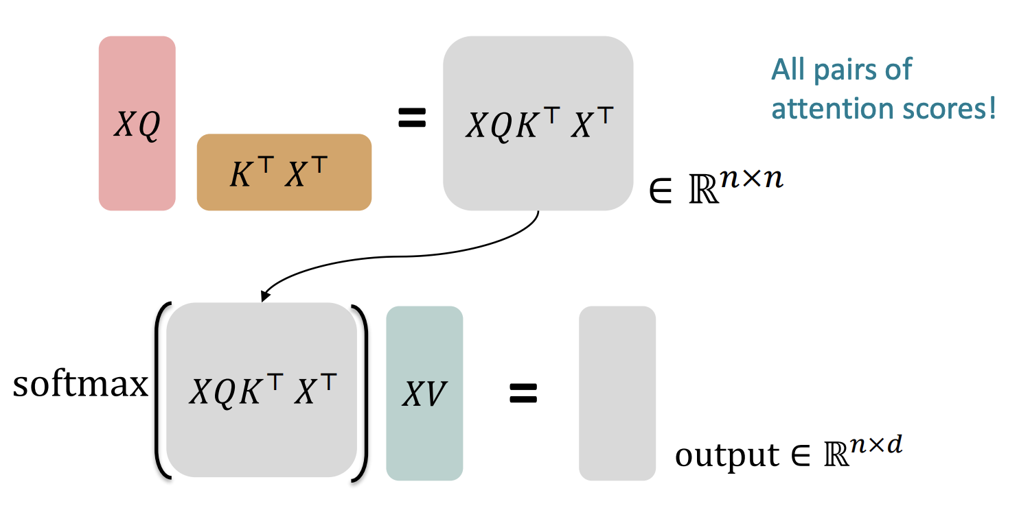
For self-attention on matrices:

• Let $X=[x_1,x_2,\dots ,x_n]\in {\mathbb{R}}^{n\ast d}$ be the input sequence.
• Let $Q,K,V\in {\mathbb{R}}^{d\ast d}$ be the query, key, and value matrices.
• This means that $XQ,XK,XV\in {\mathbb{R}}^{n\ast d}$.
• Output is $O=\text{softmax}(XQ(XK{)}^T)XV$.
  • First get attention weights by taking dot product of query and key for each word. (This is $XQ(XK{)}^T=XQ(K^T{X}^T)\in {\mathbb{R}}^{n\ast n}$). This gets all pairs of attention scores
  • Next, perform softmax on each row to get attention weights for each word. Then multiply each row by the value matrix to get the final output. (This is $O=\text{softmax}(XQ(XK{)}^T)XV$) For Multi-Head Self-Attention:
• Let $X=[x_1,x_2,\dots ,x_n]\in {\mathbb{R}}^{n\ast d}$ be the input sequence.
• Let $Q_l,K_l,V_l\in {\mathbb{R}}^{d\ast \frac{d}{h}}$ be the query, key, and value matrices for the $l$ th head, where $h$ is the number of heads, and $l$ ranges from 1 to $h$.
• Each head performs its own self-attention independent of each other
  • $O_l=\text{softmax}(X{Q}_l(X{K}_l{)}^T)X{V}_l$, where $O_l\in {\mathbb{R}}^{d\ast \frac{d}{h}}$.
• At end, all outputs are concatenated to get final output $O\in {\mathbb{R}}^d$.
  • $O=[O_1,O_2,\dots ,O_h]\in {\mathbb{R}}^d$

Scaled Dot-Product Attention §

• As the dimensionality of vector increases, dot product value gets very large, which leads to large softmax values, which leads to very small gradients, which leads to vanishing gradients.
• To solve this, we scale the dot product by $\frac{1}{\sqrt{\frac{d}{h}}}$.
• Final output is $O_l=\text{softmax}(\frac{X{Q}_l(X{K}_l{)}^T}{\sqrt{\frac{d}{h}}})X{V}_l$.

Residual Connections §

• A trick to help models train better where instead of having $X^i=F(X^{i-1})$, we have $X^i=X^{i-1}+F(X^{i-1})$.
• This allows for better gradient flow and helps with vanishing gradients or exploding gradients.

Layer Normalization §

• Within each layer, you want to get rid of uninformative variances in the model outputs, so you normalize the outputs of each layer so that they have mean 0 and variance 1.

$output=\frac{input-\mu }{\sigma -ϵ}\ast \gamma +\beta$

• $\gamma$ and $\beta$ are learned parameters that are optional

• Here is the final Decoder Transformer Layer:

Encoder Transformer Layer §

• The encoder is almost identical but without the masked self-attention layer.

Encoder-Decoder Transformer §

• You put the encoder and decoder together to get the final transformer model.
• One final difference, you have a cross-multi-head attention layer between the encoder and decoder.
• The decoder layer is the queries, and the encoder layer is the keys and values.
  • Let $h_1,h_2,\dots ,h_n$ be the hidden states of the encoder.
  • Let $s_1,s_2,\dots ,s_n$ be the hidden states of the decoder.
  • The keys and values are $k_i=K{h}_i$ and $v_i=V{h}_i$.
  • The queries are $q_i=Q{s}_i$.

Lecture 6: Pretraining §

Subword Models §

• Current assumption is that we have a fixed vocabulary of words and finite vocabulary.
• For words such as hat and tasty, you will have an embedding for each word.
• However, there can be variations of words (e.g. a typo (tsaty), a new word (tastylicious), etc.). With fixed vocabulary, there will be no mapping for these words, but you should have all the data you need to learn representations for these words.
• Current fix is to just map to an unknown token, but this is not ideal.
• Many languages have complex morphologies, which would require a very large vocabulary to cover all possible words.

Byte Pair Encoding §

• Learn vocabulary of subword units/parts of words
• Byte Pair Encoding (BPE) is a simple algorithm that learns the vocabulary of subword units.
  1. Initialize vocabulary with all characters in the training data and special end-of-word token.
  2. Using corpus of text, find the most frequent pair of characters and add them as a single unit into the vocabulary.
  3. Repeat step 2 until you reach a certain vocabulary size.
• Example: taaaaasty $\to$ taa## aaa## sty.
  • ## means that we haven’t reached the end of the word yet.
• All subwords tokens are processed identically, so there is no distinction between subwords and words.
• Long words could be broken down into many subwords if it doesnt appear often in the corpus.

Pretraining §

“the complete meaning of a word is always contextual, and no study of meaning apart from a complete context can be taken seriously.” - Firth (1935)

What we had before: Pretrained Word Embeddings §

• Around 2017:
  • Pretrained word embeddings were the standard (e.g. word2vec, GloVe, etc.)
  • Incorporate LSTM or Transformer on top of the pretrained word embeddings.
• Some issues:
  • downstream tasks will require context-specific word embeddings. (e.g question answering)

What we want: Pretrained Whole Models §

• Have all parameters in NLP models to be initialized via pretraining
• Pretraining methods hide parts of the input from the model and ask it to predict the missing parts.
• This allows:
  • Strong initialization of parameters
  • Strong representation of language.
• What can we learn from reconstructing the input?
  • Syntax (“I put ____ fork down on the table”)
  • Semantics (“I went to the ocean to see seals, fish, _____“)
  • Pragmatics
  • World Knowledge (“Stanford University is located in _______, California”)
  • Discourse
  • etc.

Pretraining with Language Modeling §

• Model $p_{\theta }(w_t|w_{1:t-1})$ by maximizing the log-likelihood of the training data.
• Save the network parameters $\theta$.
• Lots of data for this (in English at least)

Pretraining and Finetuning Paradigm §

• Pretrain a model on a large corpus of data to learn from lots of text general things. Serves as initialization.
• Finetuning on your specific task. Not as much data, but you adapt to your task. Loss converges much faster. Have to format your finetuning data to match format and task of pretraining data.

Pretraining Methods §

Encoders §

• get bidirectional context to learn representations of words
• Can’t do language modeling with bidirectional context.
• Because of this, we use masked language modeling.

Masked Language Modeling §

• Replace some fraction of the input tokens with a special mask token.
• Predict the original value of the masked tokens.
• Similar to language modeling, but you have to predict the masked tokens instead of the next word.
• For loss, only compute loss on the masked tokens.
• Example: “I went to the [MASK] and bought a [MASK] of milk.”
  • Masked tokens are “store” and “gallon”.
  • Predictions are “store” and “gallon”.
  • Loss is only computed on “store” and “gallon”.
• Used for BERT.
  • Mask out 15% of the tokens.
  • 80% of the time, replace the masked token with the mask token. (This is to prevent the model from just learning to predict the masked token)
  • 10% of the time, replace the masked token with a random token.
  • 10% of the time, keep the masked token the same.
  • This is to make sure model doesn’t just learn to predict the masked token, and it builds strong representations of all words

Next Sentence Prediction §

• Given two sentences, predict whether the second sentence is the next sentence of the first sentence.
• This would teach network long range dependencies and long distance coherence.
• Used for BERT.
• Later found that this is not necessary for good performance.

The main idea is, we are coming up with hard problems for models to solve that require the model to learn a lot of things about language.

On a bunch of NLP tasks, where models were meticulously built with special architectures and features, BERT outperformed them all in all tasks.

Limitations of Pretraining Encoders §

• Pretraining encoders is not enough for some tasks.
• You cannot use encoders for tasks that require generation (e.g. Summary Generation, Machine Translation, etc.)
• It is good for classification tasks, but not for generation tasks.

Lightweight Fine-Tuning vs Full Fine-Tuning §

• You can finetune entire models, or you can freeze some of the layers and only finetune the top layers.
• Prefix Tuning:
  • Freezes all layers, adds a prefix of parameters, and learn the prefix parameters.
• Low Rank Adaptation (LoRA):
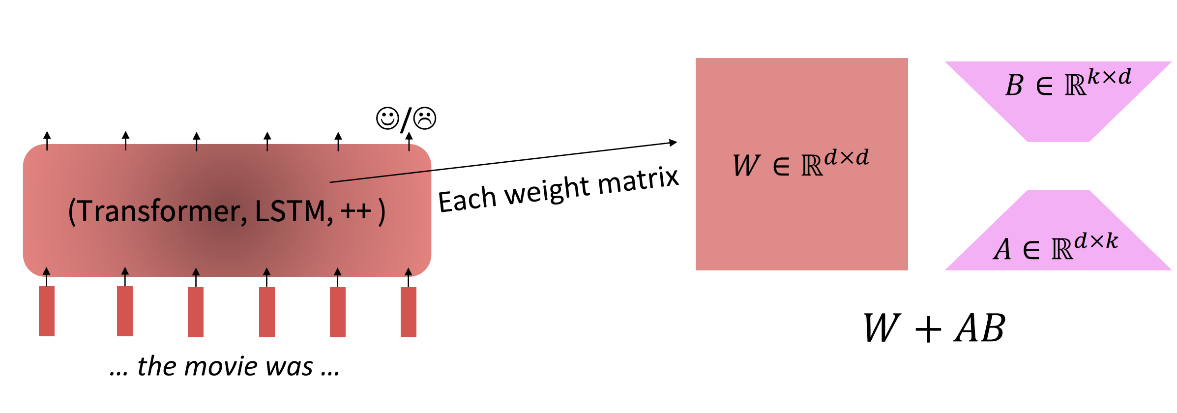
  • Learn a low rank matrix “diff” between the pretrained model and the finetuned model.

Encoder-Decoder Pretraining §

• You could do language model pretraining by splitting text into two parts and predicting the second part given the first part.
• The most optimal way to pretrain is using Span Corruption (T5) model.
  • Take a text, mask out different spans of text and predict the masked spans.
• Was very good at question answering, it was a lot better at retrieving knowledge from its pretrained knowledge base (T5)

Decoders §

• Normal language models
• Predict next word given previous words
• You add a linear layer at the end if you want to perform classification that needs to be trained from scratch.
• Majority of new models are decoders because of their simplicity and flexibility.
• Example is GPT family of models.
• When we got to GPT-3, it was a much larger model, and it could learn some tasks zero or few shot. (in context learning)

Scaling Efficiency §

• Cost of training Large Language Models is very high.
• Cost is related to number of parameters and number of tokents trained on. What is the best balance between the two?

Lecture 7: Prompting and Reinforcement Learning from Human Feedback §

Effects of Larger Models §

• We are training larger and larger models with tons of more data
• With pretraining with tons of data, you will learn a lot about a lot of things (e.g. syntax, semantics, pragmatics, etc.)
• Pretraining these large models on so much raw text data leads them to be rudimentary “world” models able to model beliefs and actions.
• Models are also exposed to lots of other data such as math, code, and encyclopedic knowledge that allows them to learn about the world and do things.
• Potential of this is using LLMs to act as assistants to humans.

Zero Shot Learning and Few Shot Learning §

Emergent Abilities of GPTs §

• The original GPT in 2018 showed that pretraining by language model training on a corpus of books is effective for other downstream tasks like natural language inference (117M Parameters).
• GPT-2 was same architecture as GPT but lot more data and larger model. Trained on internet text data. (1.5B Parameters)
  • Key takeaway: Language Models are Unsupervised multitask learners, which means they can do zero shot learning.
  • Emergent Zero Shot Learning:
    • Model can do many tasks without any finetuning or any examples. You would simply:
      • Specify the right sequence prediction problem.
        • e.g. Question Answering “Passage: Tom Brady … Question: Where was Tom Brady born? Answer:”
      • Classifiction tasks: Compare different probabilities of different sequences.
        • “The cat could not fit into the hat because it was too big”. Does “it” refer to the cat or the hat?
        • You compare P(… because the hat was too big) and P(… because the cat was too big).
    • GPT-2 was able to outperform SOTA on many tasks without any finetuning.
    • Interesting Zero-Shot behavior if you are creative enough to come up with the right prompt.
      • e.g. Summarization: Append “TL;DR:” to the end of the text to prompt the model to summarize it.
• GPT-3 was same architecture but even larger and even more parameters (175B Parameters)
  • Key takeaway: Language Models are few shot learners.
  • Specify a task by giving a few examples before your actual prompt, and then you ask model to complete the task.
  • There is a 10% accuracy increase just by adding one example to the prompt.
  • Few shot learning is an emergent property of scale
  • As you increase the number of parameters, you get better and better few shot learning.
  • Limitations:
    • Some tasks are hard to learn even with examples: e.g. Addition.
    • Mainly tasks that involve multiple steps of reasoning that even humans struggle with.
  • Chain of Thought Prompting:
    • You add reasoning to your prompt to help the model learn how to do the task.
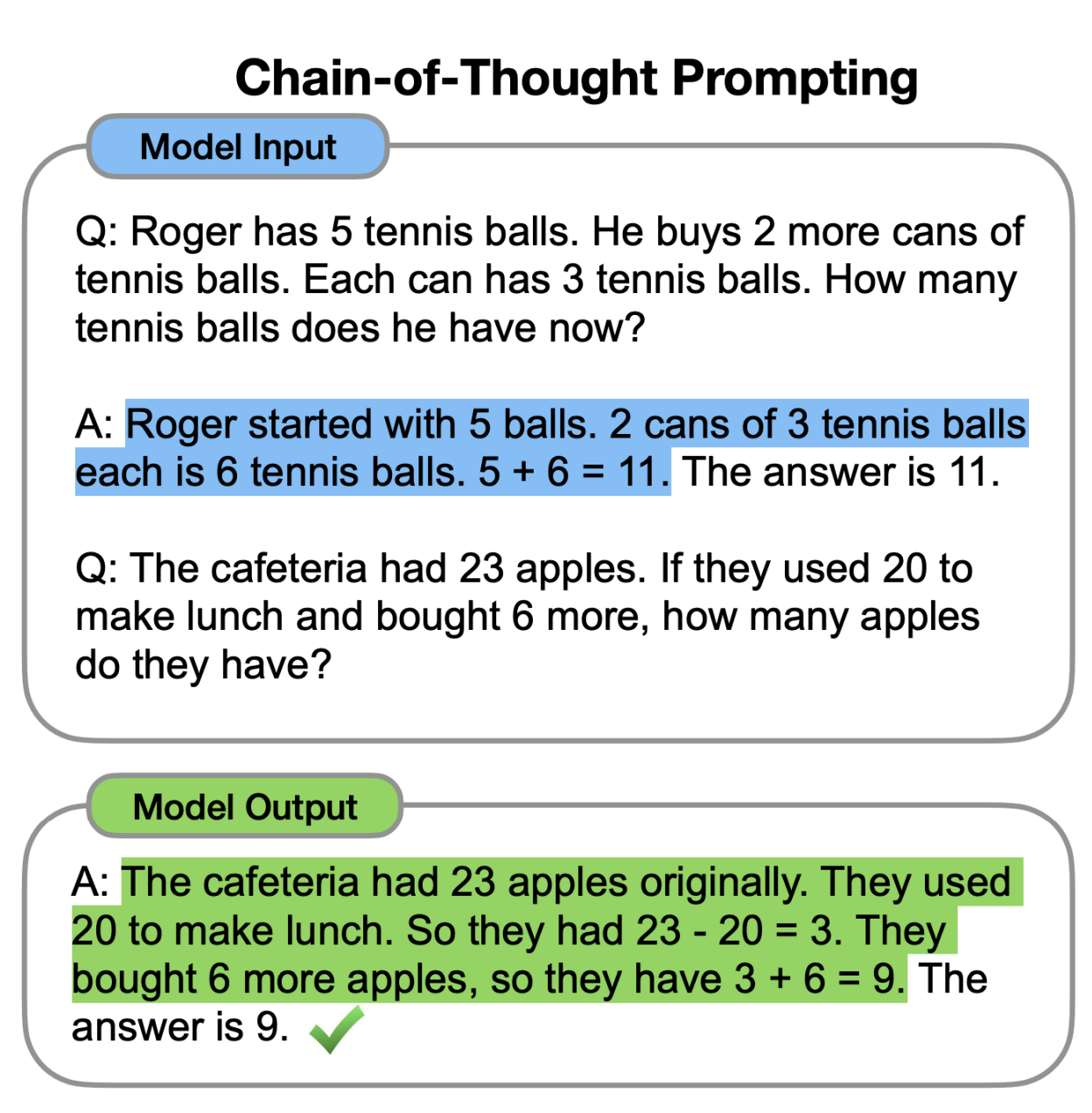
    • Allows for math problems to be easier.
    • basically providing how the model should think about the problem
  • Zero-Shot Chain of Thought:
    • Instead of adding examples of reasoning to help the model, simply ask the model to reason through the problem.
    • Performs worse than manual chain of thought, but you still get great performance.
    • Best prompt is “Lets work this out in a step by step way to make sure we have the right answer”.
• Prompt Engineering
  • Can allow you to “jailbreak” models to make the models output stuff in a way that you want.
• With prompt engineering, you are limited by the sequence length and complex tasks

Instruction Finetuning §

• Language models != assisting users
• The task given to language models is to predict the next word, which is not always aligned with user intent.
• How to align language model with user intent?
  • Collect human generated outputs for many tasks for different instructions, and then finetune the model on these instructions.
• Scale and amount and variation of data is important for this.
• This is still somewhat finetuning.
• Instruction finetuning worked for the T5 model
• Very simple to do and generalizes for many tasks.
• It is hard to get human labels to the scale that is needed. Also, humans may disagree on what the correct output is.
• Language models penalize all token mistakes equally, but some errors are worse than others.
  • “Avatar is an adventure TV show” and “Avatar is a fantasy musical” are both wrong because Avatar is fantasy more than adventure, and it is a TV show not a musical, but the musical is a far worse error than calling it an adventure show, but the model doesn’t know that

Reinforcement Learning from Human Feedback §

• Imagine training a LM on summarization:
  • For each LM sample $s$, imagine a way to obtain a human reward $R(s)\in \mathbb{R}$, where higher is better.
  • Have a human rate all summaries, where higher is good, lower is bad
  • We want to maximize the expected reward of our LM samples:
    • ${\mathbb{E}}_{\hat{s}\sim p(s)}[R(\hat{s})]$
    • As we take samples from our LM, we want the samples to maximize the expected reward.
• Using Reinforcement Learning (RL)
  • Emergence of using RL with LMs
  • Newer RL algorithms make it possible to integrate RL with LLMs
• How to update our parameters $\theta$ to optimize for human preference:
  • ${\mathbb{E}}_{\hat{s}\sim p(s)}[R(\hat{s})]$
  • Since we maximize the above formula, try to use gradient ascent to maximize it.
  • ${\theta }_{t+1}:={\theta }_t+\alpha {\nabla }_{{\theta }_t}{\mathbb{E}}_{\hat{s}\sim p(s)}[R(\hat{s})]$
    • How do we estimate the expectation, and what if the reward function is not differentiable?
  • We use policy gradient methods in RL to give us tools to perform the gradient ascent.
    • ${\nabla }_{\theta }{\mathbb{E}}_{\hat{s}\sim p(s)}[R(\hat{s})]={\nabla }_{{\theta }_t}{\sum }_{s}R(s)p_{\theta }(s)={\sum }_{s}R(s){\nabla }_{{\theta }_t}{p}_{\theta }(s)$
    • Using log-derived trick to take derivative of $\log p_{\theta }(s)$, we get:
      • ${\nabla }_{{\theta }_t}\log p_{\theta }(s)=\frac{{\nabla }_{{\theta }_t}{p}_{\theta }(s)}{p_{\theta }(s)}$
      • ${\nabla }_{{\theta }_t}{p}_{\theta }(s)=p_{\theta }(s){\nabla }_{{\theta }_t}\log p_{\theta }(s)$
    • We can now rewrite the gradient as:
      • ${\nabla }_{\theta }{\mathbb{E}}_{\hat{s}\sim p(s)}[R(\hat{s})]={\sum }_s{p}_{\theta }(s)R(s){\nabla }_{{\theta }_t}\log p_{\theta }(s)$
    • We see that the right-hand side is an expectation, so we can rewrite it as:
      • ${\mathbb{E}}_{\hat{s}\sim p_{\theta }(s)}[R(\hat{s}){\nabla }_{{\theta }_t}\log p_{\theta }(s)]$
    • The gradient is now inside the expectation, which means we can approximate it using Monte Carlo sampling.
      • ${\nabla }_{\theta }{\mathbb{E}}_{\hat{s}\sim p(s)}[R(\hat{s})]\approx \frac{1}{N}{\sum }_{i=1}^{N}R({\hat{s}}_i){\nabla }_{{\theta }_t}\log p_{\theta }({\hat{s}}_i)$
    • We then get the following update rule:
      • ${\theta }_{t+1}:={\theta }_t+\alpha \frac{1}{N}{\sum }_{i=1}^{N}R({\hat{s}}_i){\nabla }_{{\theta }_t}\log p_{\theta }({\hat{s}}_i)$
    • What does this mean:
      • Simple case:
        • Imagine reward was binary reward (0 or 1).
        • When we get a reward of 1, we are performing normal gradient ascent, but when we get a reward of 0, we do nothing (?)
      • More generally, if reward was scalar:
        • When R is very high, we multiply the gradient by a large number, so we take a large step in the direction of the gradient.
        • If R is low and negative, we multiply the gradient by a negative number, so we take a large step in the opposite direction of the gradient to decrease the probability of the sample.
• Limitations:
  • Again, expensive and not scalable to get humans to rate all samples.
    • Solution: Train another NLP model that will model human preferences and spit out a reward for each sample.
  • Human preferences can be noisy and miscalibrated.
    • Solution: ask humans to compare two samples and tell you which one is better, which makes it more reliable.
    • The NLP model that models human preferences will also be trained on these pairwise comparisons.
• Putitng it all together:
  • We have a pretrained LLM that may also be instruction finetuned $p^{PT}(s)$.
  • We have a reward model $R{M}_{\varphi }(s)$ producing scalar rewards for LLM outputs trained on human preferences dataset
  • We have a method to optimize LLM parameters towards a reward function.
  • To do RLHF:
    • Clone pretrained model $p^{PT}(s)$ to get $p_{\theta }^{RL}(s)$.
    • Optimize the following reward using RL:
      • $R(s)=R{M}_{\varphi }(s)-\beta \log \frac{p_{\theta }^{RL}(s)}{p^{PT}(s)}$
      • The second term is a penalty to make sure we do not stray too far from the pretrained model. (KL Divergence)
      • $\beta$ is a hyperparameter that controls how much we want to penalize the model for straying too far from the pretrained model.
• InstructGPT:
  • Scale up RLHF to tens of thousands of tasks
• Using RLHF helps align the model more with human preferences instead of just focusing on the next word prediction task.
• It is hard to get right using RL.
• Human Preferences are unreliable:
  • Chatbots are rewarded to produce responses that seem authoritative and helpful, whether or not the information is actually true or not

  It is naive to think that all of human preferences for a task can be captured by a single scalar reward function.

• RLHF being the main driver in aligning models with human preferences can have issues because of the unreliability of human preferences and reward hacking.