Backpropagation

Before reading this, make sure to read the piece on Gradient Descent, as this will build off of that piece.

Motivation §

From the gradient descent article, we saw that given input data $X$ and output data $Y$, we can approximate parameter values/matrices such as $W$ and $b$ that would best map data points in $x_i$ to their corresponding outputs $y_i$ using an iterative algorithm that would aim to minimize a loss/cost function. We would find the gradient of the cost functions with respect to our parameters (in this case $W$ and $b$), and slowly descend towards a local minimum with the following equation:

${\Theta }_{new}={\Theta }_{old}-\alpha \nabla (J(\Theta ))$

where $\alpha$ is a hyperparameter of the learning rate. Computing the gradient for each parameter in this case does not require much effort, as there are no complex functions, and there aren’t a significant amount of parameters to account for. However, consider the following picture:

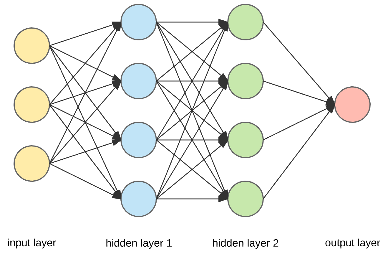
Here we see 4 layers: the input, 2 hidden layers, and the output layer. Each component of the input layer is sent to all 4 of the nodes in the first hidden layer, and each node in the first hidden layer is passed to each node in the second hidden layer etc. At each node, except for the input, the input data into the node is first transformed linearly, similar to $Wx+b$. However, the input is then transformed with some nonlinear function. We can see here that the amount of parameters greatly increases as our machine learning architectures become more complex. Each node in hidden layer 1 has weights associated with each input node, and each node in hidden layer 2 has weights associated with each node in hidden layer 1. Additionally, the nonlinearities add another level of complexity. We can see that as the complexity of the architecture increases, it becomes more and more computationally expensive to go and calculate the gradient of every single parameter of the network individually. So, how can we do this in an efficient way such that we don’t lose as much time calculating all the gradients.

The Chain Rule §

Before we get into the algorithm, we visit a topic from calculus that is the foundational building block of the algorithm: the chain rule. Say we have a function $f(x)$, and then a function $g(f(x))$, and we wanted to find the derivative of $g$ with respect to $x$. We would first take the derivative of $g$ with respect to $f$, and then multiply it by the derivative of $f$ with respect to $x$. In other words:

$\frac{\mathrm{d}g}{\mathrm{d}x}=\frac{\mathrm{d}g}{\mathrm{d}f}\ast \frac{\mathrm{d}f}{\mathrm{d}x}$

As you can, when we compound functions, we begin multiplying derivatives in order to calculate the full derivative. We can leverage this when calculating gradients for deep neural networks.

Applying the Chain Rule to Neural Network Gradient Descent §

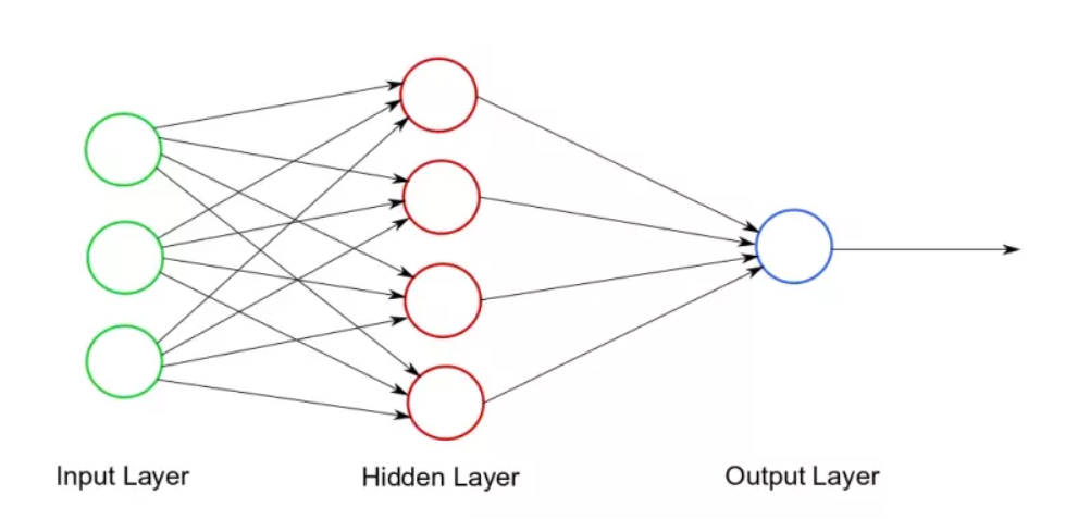
Consider the following neural network: We have 4 total layers: one input layer, 2 hidden layers, and one output layer. The inputs normally are multidimensional feature vectors. This feature vector is fed into each node in the first hidden layer. In each node of the first hidden layer, there exists a set of parameters $W$ and $b$. These parameters allow us to perform a linear transformation on the feature vector $x$, creating $z=Wx+b$. Since $x$ is multidimensional, and each input node is connected to each hidden layer node, $W$ and $b$ both end up being matrices containing multiple parameters. After performing the linear transformation, the hidden layer performs a nonlinear transfer function $y=h(z)$. This becomes the output of the hidden layer. It also becomes the input of the next hidden layer. In the next hidden layer, the same process takes place, but with different $W$ and $b$ matrix values. This is repeated until we get to the output layer, where we finally get the final values.

Clearly with the fully connected network of neurons, and all the weights and biases associated with each neuron, and the nonlinearity applied at each neuron, calculating the gradients of each parameter would be a very cumbersome and computationally expensive process. However, we can greatly expedite this process using the chain rule. Going through the network, we can see that all we are really doing is repeatedly compounding functions onto the original input layer. We take the input, we call $x_0$, and we pass it into the first hidden layer, where we perform a linear transformation:

$z_1=W_1{x}_0+b_1$

We then take this result, and perform a nonlinear transfer function on it to get the output of the layer:

$x_1=h(z_1)$

This also becomes the input of the next layer. We continuously compound more and more functions on top, producing more parameters the more layers we have.

This situation lends itself to the chain rule naturally, and we will be able to leverage the chain rule to more efficiently calculate the gradients.

The Algorithm §

To understand the algorithm, lets look at a simpler neural network: Here we have the input layer, 1 hidden layer, and the output $y$. What is going to happen here? First, $x$ wil be passed into the hidden layer, and a linear transformation will be performed on it:

$z=Wx+b$

with $W$ being a weight matrix and $b$ being a bias matrix. Then, a nonlinear transfer function will be performed on it:

$h=f(z)$

This will be the output of the hidden layer. This will be inputted into the output layer, where a final function will be performed on the input:

$s=u(h)$

and this will be our final output. Now, let’s say we want to find $\frac{\partial s}{\partial b}$. To get to the parameter $b$, we have to go from the output function, back to through the output function and the nonlinear transfer function. By the chain rule, we then get that:

$\frac{\partial s}{\partial b}=\frac{\partial s}{\partial h}\frac{\partial h}{\partial z}\frac{\partial z}{\partial b}$

This will get us the gradient with respect to $b$. Now, let’s say we want to find the gradient with respect to $W$, the weight matrix. Again, we first have to go through the output function and the nonlinear transfer function. With the chain rule, we get:

$\frac{\partial s}{\partial b}=\frac{\partial s}{\partial h}\frac{\partial h}{\partial z}\frac{\partial z}{\partial W}$

We can see that in both calculations, we have a commonality in $\frac{\partial s}{\partial h}\frac{\partial h}{\partial z}$, so calculating the gradient for both parameters would result in duplicate computation. The backpropagation algorithm is made to avoid making these duplicate computations. Take the equation stack from before:

$$\begin{gathered} s=u(h) \\ \downarrow \\ h=f(z) \\ \downarrow \\ z=Wx+b \\ \downarrow \\ x. \end{gathered}$$

The idea is that at each level in the stack, we want to compute something, we can call this $\delta$, that we can pass down the stack when we want to compute the gradient with respect to parameter(s) lower in the stack, and this will prevent us from making duplicate computations. At the top level, we compute ${\delta }_0$ to be $\frac{\partial s}{\partial h}$. Then, in the second layer, we compute ${\delta }_1={\delta }_0\ast \frac{\partial h}{\partial z}$. This ${\delta }_1$ will be passed down to the third layer, and can be used to calculate both $\frac{\partial s}{\partial W}$ and $\frac{\partial s}{\partial b}$: $\frac{\partial s}{\partial W}={\delta }_1\ast \frac{\partial z}{\partial W}$ $\frac{\partial s}{\partial b}={\delta }_1\ast \frac{\partial z}{\partial b}$ As you can see, the $\delta$’s allow us to store previous gradient values that we can pass back down the network to be used to calculate further gradients without repeated computations. Formally, $\delta$ in each layer is called the local error signal.

This becomes a scalable way to compute gradients of complex neural networks. As the number of layers, and the number of neurons increases, by holding the local error signal at each layer, we are still able to compute gradients efficiently.

Application in Software §

In theory, this is the backpropagation algorithm in its full form: we compute local error signals at each layer which is passed down to the lower layers to allow more efficient computation of gradients. But how is this implemented in software.

In the real world, to perform this algorithm, computation graphs are created, where source nodes are the inputs, and interior nodes are the operations: 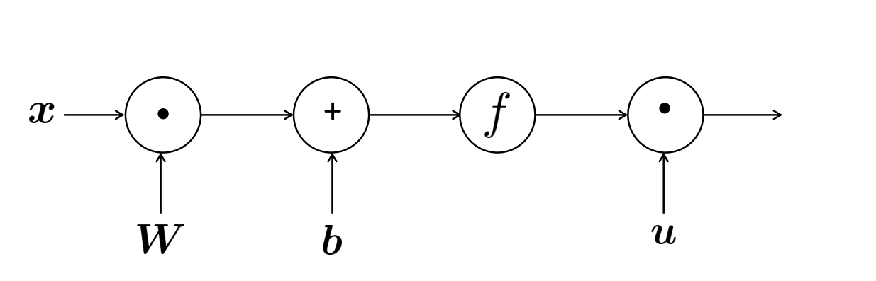This is similar to an expression tree. When determining the value of the output, this graph is evaluated identically to an expression tree. This differs, though, because at each node, we are able to store the local gradient at that node, which will be propagated back to all the nodes behind it, allowing us to calculate the gradients for each source node that will be used to update the parameters.

Summary and Final Thoughts §

This is the backpropagation algorithm in full. We store local error signals at each layer of the stack and pass them down the stack to allow us to compute gradients efficiently enough so we can update parameters of complex neural networks with adequate efficiency. This algorithm stands out to me so much because it requires extensive knowledge of concepts in both calculus and software engineering. In my head, the storing of local error signals reminds me of dynamic programming, similar to memoization. Additionally, creating computation graphs and expression trees is a foundational software engineering principle. The intersection of math and software engineering here makes a very elegant algorithm in my opinion.