Sorting with ODEs

This semester I’m taking a course on unconventional computation techniques, and one of the topics we covered was analog computation. Analog computers are a type of computer that use continuous physical phenomena like electrical, mechanical, or even chemical processes to model and solve problems. The main “programming language” for these computers is differential equations, more specifically, systems of polynomial ordinary differential equations (ODEs).

Through this paper, it can be proven that any discrete algorithm solved in polynomial time can be solved via a system of polynomial ODEs also in polynomial time.

An example of this is sorting, more specifically, bubble sort. If you are not familiar with bubble sort, it is a simple sorting algorithm that repeatedly steps through a list, compares adjacent elements and swaps them if they are in the wrong order. The pass through the list is repeated until the list is sorted.

Surprisingly, bubble sort can be solved using a system of ODEs.

ODE for swapping two elements §

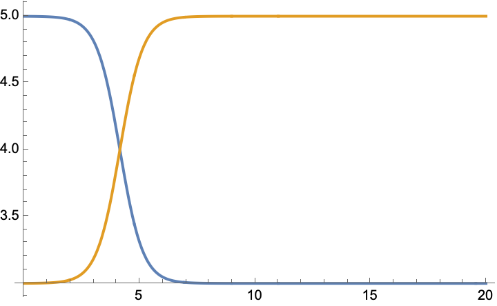
The first step is to model the swapping of two elements in a list. Let’s say we have two elements $X_1$ and $X_2$, and we want to order them such that $X_1\le X_2$. We can model the swapping of these two elements using the following ODE:

$X_1^{\prime }=-Y$

$X_2^{\prime }=Y$

$Y^{\prime }=(X_1-X_2)Y$

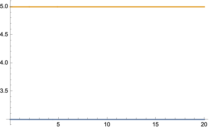
With this system of equations, if $X_1>X_2$, then $X_2$ will grow to the value of $X_1$ and $X_1$ will decay to the value of $X_2$ as shown: If $X_1<X_2$, then the values will stay constant as shown: The best way to understand this system is to understand the following differential equation: $X^{\prime }=aX$ where $a$ is a constant. The solution to this equation is $X(t)=X(0)e^{at}$, so when $a$ is positive, $X$ grows exponentially, and when $a$ is negative, $X$ decays exponentially. This intution can be used to understand the $Y$ variable and how it affects the $X_1$ and $X_2$ variables. The $Y$, which initially starts at a really small positive value, acts as a “force” variable that controls the swapping of the $X_1$ and $X_2$ variables. $(X_1-X_2)$ acts similar to the $a$ constant. If $X_1<X_2$, then $(X_1-X_2)$ is negative, and $Y$ will decay to zero, and since it is a small positive value, it will decay super fast to zero, leaving the $X_1$ and $X_2$ variables unchanged. However, if $X_1>X_2$, then $(X_1-X_2)$ is positive, and $Y$ will grow, driving the $X_1$ down (because $X_1^{\prime }=-Y$) and the $X_2$ up (because $X_2^{\prime }=Y$).However, as $X_1$ and $X_2$ get closer, the $(X_1-X_2)$ value will get smaller, the rate at which $Y$ grows will get smaller, until $X_1=X_2$, which is the point of inflection. After this point, $X_1$ will be less than $X_2$, so $(X_1-X_2)<0$, so $Y$ will start to decay. This will cause the rate at which $X_1$ is decreasing and $X_2$ is increasing to decrease, until they both stop changing, which is the point of equilibrium, as shown in the first graph.

Here is the graph of the values swapping with $Y$ also plotted: 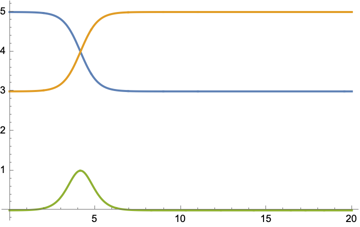You can see that $Y$ grows when $X_1>X_2$ and decays when $X_1<X_2$.

ODE for bubble sort §

Now that we have the ODE for swapping two elements, we extend this to another ODE to model bubble sort for a list of 3 elements: $X_1^{\prime }=-Y_1$ $X_2^{\prime }=Y_1-Y_2$ $X_3^{\prime }=Y_2$ $Y_1^{\prime }=(X_1-X_2)Y_1$ $Y_2^{\prime }=(X_2-X_3)Y_2$ This system of equations models sorting 3 elements such that $X_1\le X_2\le X_3$. The $Y_1$ is the “force” variable between elements $X_1$ and $X_2$, and $Y_2$ is the “force” variable between elements $X_2$ and $X_3$. So for $X_2^{\prime }$, it must have positive $Y_1$ to make sure it is greater than $X_1$, and it must have negative $Y_2$ to make sure it is less than $X_3$. The $Y_1$ and $Y_2$ variables are the “forces” that drive the elements to their correct positions.

Here is an example where the list is $[3,5,1]$, or in our case $X_1(0)=3,X_2(0)=5,X_3(0)=1$. We want the end result to be $[1,3,5]$, or $X_1(\infty )=1,X_2(\infty )=3,X_3(\infty )=5$. Here is the graph of the values swapping:

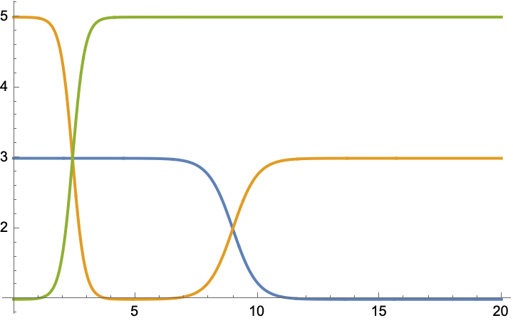
You can see that first $X_2$ and $X_3$ swap, but $X_1$ is idle, because from the information it has (only $X_1$ and $X_2$), it sees that it is in the correct position. However, once $X_2$ and $X_3$ swap, then $X_1$ and $X_2$ need to swap to get the correct order.

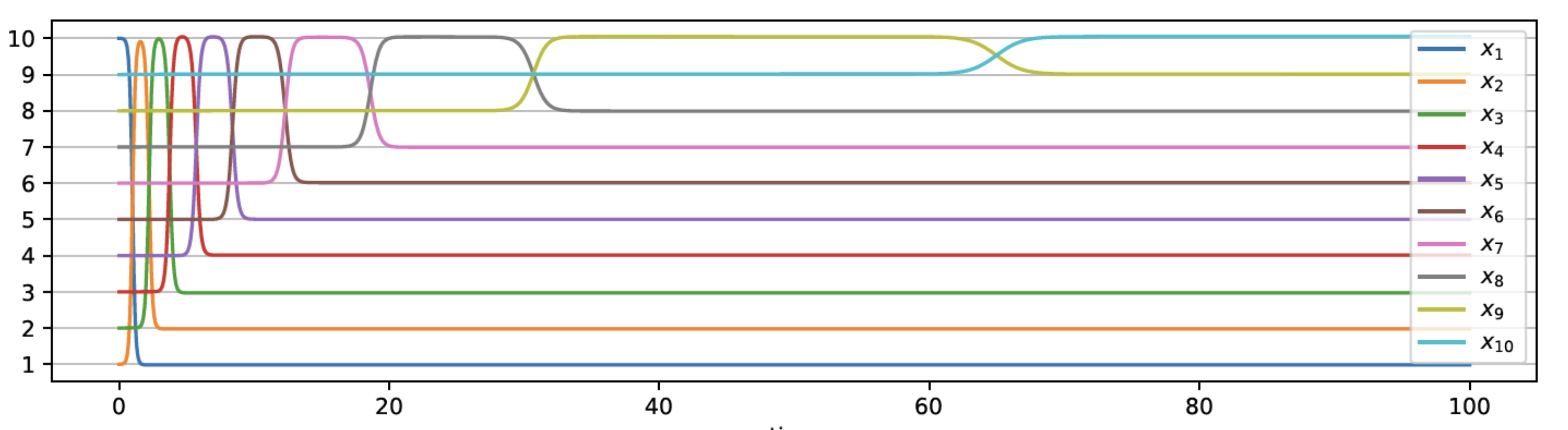
This can extend to any number of elements $n$, as shown in this graph of sorting 10 elements:

Though this is not necessarily a practical way to perform computation at scale at the moment, I still think it is pretty cool you can take a discrete algorithm that is more of an abstract concept and model it using polynomial ODEs.