Stochastic Gradient Descent

What is Gradient Descent? §

Gradient descent is an iterative first order optimization algorithm that is used to find local minima (or maxima) of functions. While there are many applications for this algorithm, probably the most notable is its applications in machine/deep learning.

What is a gradient? §

First, we define what a gradient is. For a univariate function, the gradient is simply the first derivative of the function. So for example if we have the function $y=x^3$, we can say that the gradient at point is $\frac{\mathrm{d}y}{\mathrm{d}x}=3x^2$. Now, if we extend this to a multivariate function of $n$ variables with one output, $f(x_1,x_2,\dots ,x_n)$ the gradient would be an n-dimensional vector with the $i$th entry being the partial derivative of f with respect to $x_i$:

$\nabla (f)=\left[\begin{array}{c}\frac{\partial f}{\partial x_1}\\ \frac{\partial f}{\partial x_2}\\ ⋮\\ \frac{\partial f}{\partial x_n}\end{array}\right]$

This can be further extended to a multivariate function with $m$ outputs, which would create an $n\ast m$ matrix, with each column $i$ being all the partial derivatives for output $y_i$. The gradient defines the direction of the greatest/fastest increase in the function at a point. This also means that the negative gradient would be the greatest/fastest decrease in the function at a point, and it is this fact that we leverage in order to use gradient descent for to train machine learning models.

The Algorithm §

Lets consider the linear regression problem, as this is the simplest to understand. We have input data $X$, where each entry can be an $n$ dimensional vector, and output data $Y$ (also can be multiple dimensions), and we would like to find a line that would best model the relationship between $X$ and $Y$. $y^{\prime }=Wx+b$ where $y^{\prime }$ is the predicted value, $W$ is the slope of the line, and $b$ is the intercept. However, with only the input data, output data, and infinite possibilities for $W$ and $b$ how can we possibly find the optimal values of $W$ and $b$? We first define a loss function, which basically is a function that measures how wrong a machine learning model is from ground truth. For different problems, there are different loss functions, so to be general, we will simply call it $J(y,y^{\prime })$, where $y$ is the ground truth and $y^{\prime }$ is the predicted value. We know $y^{\prime }$ is a function of $W$ and $b$, so we actually have the loss function being $J(y,W,b)$, where $W$ and $b$ are parameters of the linear function. Our goal will be to minimize the loss function, and since we can only change $W$ and $b$, we will consider the loss function to only be a function of $W$ and $b$, $J(W,b)$. We can use gradient descent with $W$ and $b$ being the input variables to minimize this function.

The algorithm is as follows (We represent $W$ and $b$ as $\Theta$, the set of parameters of the function):

${\Theta }_{new}={\Theta }_{old}-\alpha \nabla (J(\Theta ))$

In terms of $W$ and $b$:

$W_{new}=W_{old}-\alpha \frac{\partial J}{\partial W}$ $b_{new}=b_{old}-\alpha \frac{\partial J}{\partial b}$

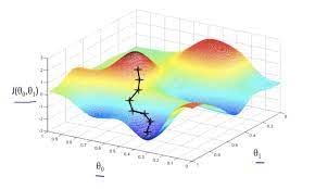
Now, we dissect this formula. We take our current point, find the direction of steepest descent, and we take a scaled step in that direction, with $\alpha$ being the scaling factor (also called the learning rate). $\alpha$ is what we call a hyperparameter whose value is determined by the user. At each time step we perform this algorithm, as we slowly make our way down to the minimum point of the loss function, and at the point of convergence (or close to it) is the values of $W$ and $b$ we use. An image is shown for a visual example:

In choosing $\alpha$, we have to be careful. If we choose a value too small, we will take a really long time to converge, and if we pick a value too big, we will never converge, as our step sizes can skip the minimum entirely.

In summary, the gradient descent algorithm is used to iteratively find the values of all parameters of a machine learning model such that the value of the loss function defined for the model is minimized.

Why use Gradient Descent §

People familiar with probability and statistics may look at this and wonder, why do we use gradient descent to find $W$ and $b$, when there are closed form equations we can use to calculate $W$ and $b$. The simple answer is that this approach simply is not scalable. When there is a large amount of data and the dimensionality of this data continues to increase, the computations needed for these closed form formulas becomes far too inefficient. Additionally, when we encounter more complex models that involve deep neural network architecture with nonlinearities, this just becomes too complex. Gradient descent is a scalable and generalizable algorithm that can produce results on the same levels of accuracy.

Stochastic Gradient Descent vs Gradient Descent §

While gradient descent is more efficient than the closed form formulas, there do exist inefficiencies. Mainly, each iteration of gradient descent does not occur until all sample data points have been run through. This means, if we have a huge dataset, it would take quite a while just to produce one iteration of gradient descent. This is where stochastic gradient descent comes in. Instead of iterating through all data points to make an update to the parameters, you only use a subset of the samples before you make an update. This involves creating batches of input data where, after going through one batch, an update is made. This allows the algorithm to converge a lot faster than normal gradient descent. However, stochastic gradient descent often does not produce as optimized results as gradient descent, which intuitively makes sense, but the results are approximate enough that the time saved is worth the decrease in optimization.

Final Thoughts §

I find gradient descent to be a fascinating algorithm for a couple reasons. First, I never thought that the concept of a derivative, something I learned at the beginning of my high school calculus class could grow into an algorithm that is central to all machine learning. Second, the way that when models deal with inputs of multiple dimensions, this algorithm can simplify much of its calculations down to fast matrix multiplication operations makes this a very elegant algorithm in my opinion.